Commodity Price Prediction (Part I)

I’ve been fascinated by the financial/trading sector since probably my mid-20s. As a part of this fascination, I wanted to use machine learning to see if we can build a model to predict commodity futures prices within a 5% error rate.

The dataset that I used in this project was the World Bank Commodity Price Kaggle dataset, spanning from 1960 to 2026. It covers the monthly price of 71 commodities across 10 broad categories. The primary source of the data is from the World Bank Pink Sheet (CMO Historical Data Monthly) which spanned to end 2024; the data from Jan 2025 - Feb 2026 was sourced from the FRED API. Since then, the link to the dataset on Kaggle broke - although the data still exists on World Bank site here. The dataset I used is still available on my GitHub repo. Since we also needed to ensure that the prices were adjusted for inflation, the target column that we are using in this project is the price_index_2000_base, and not price_nominal_usd.

As with all historically-based, sequential data, we have to use a form of time-series analysis. There are a few options here, like SARIMA (to include data-handling with recurring seasonal patterns), and some variations of LSTM-GARCH or LSTM-GBDT. During the time I was completing this project, I knew I wanted to look at differences between a naive prediction model, so I included SARIMA. However, at the time, I wasn’t aware of LSTM, so I only used the XGBoost algorithm – but in order to do so, the data needs to be transformed into a tabular, supervised learning format, which leads us to the next point.

One of the things I wanted to be cautious of was data leakage. I mitigated this by excluding the 3-, 6-, and 12-month price averages since that would include the current month’s price. In order to transform the data from sequential data to tabular data, I computed rolling lags for 3-, 6-, 12-months, which would exclude the current month’s price into the average.

Since none of the algorithms support time-series forecasting across multiple commodities (and I didn’t really see a practical reason for doing so), I trained individual models for each commodity.

For future exploration/flexibility, the config.py allows us to set specific commodities we’re interested in using COMMODITY_LIST. I also set other variables like the LAG_PERIODS, TRAIN_CUTOFF_YEAR (to specify where we’re splitting off the training/testing sets), RANDOM_SEED, XGB_PARAMS, and XGB_OPT_PARAMS.

For the purpose of this post, I chose these 3 commodities:

• Crude oil, Brent
• Natural gas, Europe
• Wheat, US HRW (Hard Red Winter)

Step 1: Load data

The loading of the CSV data into a dataframe (simply by using pd.read_csv), indexed by the date column (converted to datetime) is fairly straightforward here.

1
2
3
4
5
6
7
8

def _parse_dates(df: pd.DataFrame) -> pd.DataFrame:
    if 'date' not in df.columns:
        raise KeyError("ERROR: 'date' column was not found in the DataFrame")

    df['date'] = pd.to_datetime(df['date'])
    df.set_index('date', inplace=True)

    return df

However, since we’re specifying the commodities we’re interested in, we need to validate that the commodities we specified are in the dataframe, and split the dataframe by commodity name into smaller dataframes.

 1
 2
 3
 4
 5
 6
 7
 8
 9
10
11
12
13
14
15
16

def _validate_columns(df: pd.DataFrame) -> pd.DataFrame:
    available = df['commodity_name'].unique()
    missing = [col for col in config.COMMODITY_LIST if col not in available]

    if missing:
        print(f"WARNING: The following commodities were not found in the DataFrame and will be omitted: "
              f"{missing}")
        config.COMMODITY_LIST[:] = [col for col in config.COMMODITY_LIST if col not in missing]

    if not config.COMMODITY_LIST:
        raise KeyError(
            f'ERROR: None of the configured commodities from COMMODITY_LIST were found in the dataset.'
            f'Please check the COMMODITY_LIST param in config.py'
            )

    return df

 1
 2
 3
 4
 5
 6
 7
 8
 9
10
11
12

def _split_by_commodity(df: pd.DataFrame) -> dict[str, pd.DataFrame]:
    commodity_dfs = {}

    for commodity in config.COMMODITY_LIST:
        cdf = (
            df[df['commodity_name'] == commodity]
            .copy()
        )
        cdf = _sort_index(cdf)
        commodity_dfs[commodity] = cdf

    return commodity_dfs

Although I did inspect the original CSV file to ensure that the dates were ascending, it’s better practice to ensure this programmatically, so I wrote a small helper function called _sort_index that sorts the index if it’s not ascending.

Step 2: Preprocess data

In this step, I dropped quite a few columns from the list of dataframes; these columns were either redundant, held metadata, were auditing fields, or posed potential for leakage. I also forward-filled and then back-filled any gaps that occur at the start of the series - this order is necessary since forward-filling first prevents any data leakage and follows a chronological order. Back-filling after cleans up the remaining edge cases.

There were also a few categorical columns like quarter, decade, and era (containing values like ‘Pre-Oil Shock Era’, ‘Reaganomics Era’, and ‘COVID & Post-Pandemic Era’, etc.), so I opted to encode them so that we could use them as features in XGBoost:

 1
 2
 3
 4
 5
 6
 7
 8
 9
10
11
12
13
14
15
16
17
18
19
20
21
22

def _encode_categoricals(df: pd.DataFrame) -> pd.DataFrame:
    """
    Encodes categorical columns that have predictive value into integers so that XGBoost can use them as features
    'quarter' => integer 1-4
    'decade'  => integer (e.g., 1960, 1970, etc)
    'era'     => one hot encoded value
    """
    # quarter: 'Q1' -> 1, 'Q2' -> 2, etc.
    if 'quarter' in df.columns:
        df['quarter'] = df['quarter'].str.replace('Q', '').astype('int')

    # decade: '1960s' -> 1960; '1970s' -> 1970, etc.
    if 'decade' in df.columns:
        df['decade'] = df['decade'].str.replace('s', '').astype('int')

    if 'era' in df.columns:
        era_dummies = pd.get_dummies(df['era'], prefix='era', drop_first=True)
        era_dummies = era_dummies.astype('int')
        df = pd.concat([df.drop(columns=['era']), era_dummies], axis=1)
        print(f'era: one-hot encoded into {len(era_dummies.columns)} columns.')

    return df

Step 3: EDA (Exploratory Data Analysis)

Across each commodity, I wanted to look at the data distribution before and after preprocessing, so the EDA module takes a string param we called stage (default value=raw, unless we pass preprocessed).

In this step, we want to get the summary statistics, run an ADF (Augmented Dickey-Fuller) test, and plot both the histograms and scatter plots to inspect the data distribution. We can easily do this for all the commodities in our COMMODITY_LIST using a loop:

 1
 2
 3
 4
 5
 6
 7
 8
 9
10
11

def run_eda(commodity_dfs: dict, stage: str = 'raw') -> dict:
    for commodity, commodity_df in commodity_dfs.items():
        print_commodity_header(f"{commodity}")
        _summary_statistics(commodity_df)
        _adf_test(commodity_df, stage)
        _plot_histogram(commodity_df, commodity, stage)
        _plot_scatterplot(commodity_df, commodity, stage)

    _plot_price_history(commodity_dfs, stage)

    return commodity_dfs

I was interested in the outcomes of the ADF test since I’m still working to understand it. Across all the commodities I selected, all of them were non-stationary:

----------------------------------------
Crude oil, Brent
----------------------------------------
Stationarity (Augmented Dickey-Fuller Test):
ADF Statistic: -1.7041
p-value: 0.4290
Verdict: Non-Stationary
Data is Non-Stationary - Differencing recommended.

----------------------------------------
Natural gas, Europe
----------------------------------------
Stationarity (Augmented Dickey-Fuller Test):
ADF Statistic: -2.7720
p-value: 0.0624
Verdict: Non-Stationary
Data is Non-Stationary - Differencing recommended.

----------------------------------------
Wheat, US HRW
----------------------------------------
Stationarity (Augmented Dickey-Fuller Test):
ADF Statistic: -2.7594
p-value: 0.0643
Verdict: Non-Stationary
Data is Non-Stationary - Differencing recommended.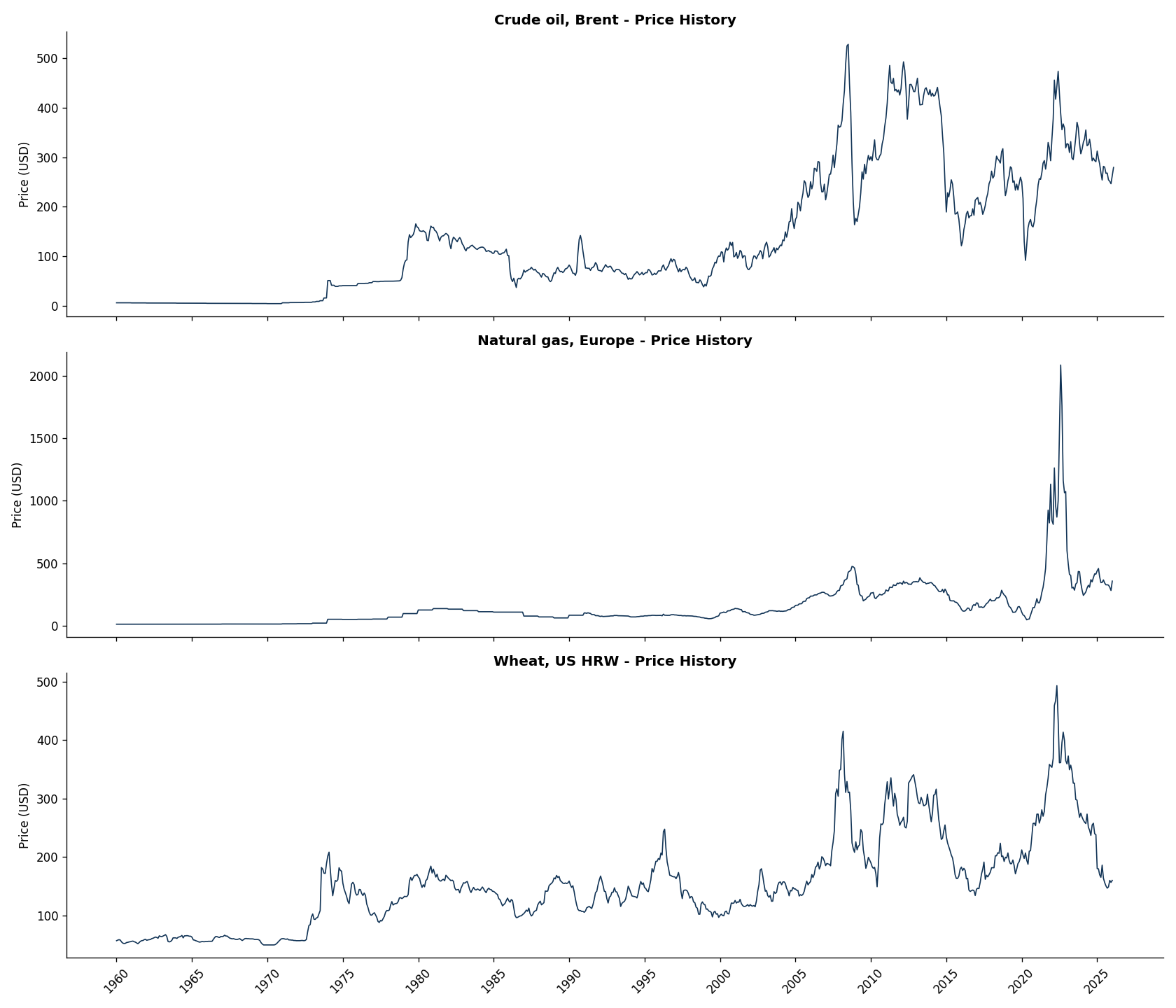

When we look at the price history graphs across commodities, we can see that there’s no strong repeating cycles in the commodity prices. There is no stationarity (ie., there is no constant mean, variance, and has changing statistical properties over time). When data is non-stationary, the mean is changing (average value goes up and down over long period); the variance is changing (the spread/scatter of data points gets smaller or larger over time). Non-stationarity matters because standard statistical models struggle to predict future values if the underlying rules keep shifting. This is important since it indicates a need for differencing/removing the trends to make the data stationary before building any models.

Each commodity’s histogram also shows right-skewedness with fat tails:

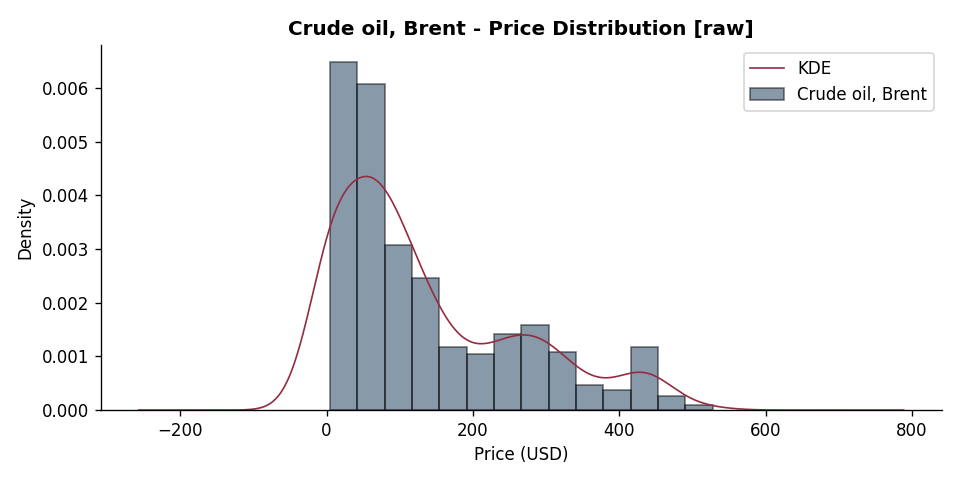
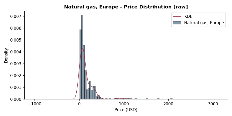
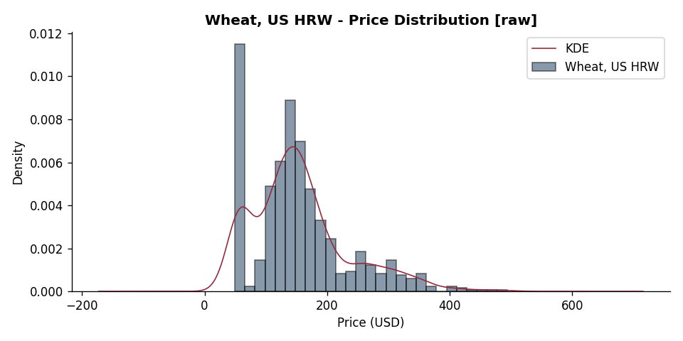
Practically speaking, we should not expect a normal distribution; commodity prices should feature positive skewness, fat tails (due to extreme market events), and non-negative boundaries (prices cannot drop below zero).

Based on the first pass of the EDA, I can think of a few transformations (e.g., transforming price_index_2000_usd into percentages rather than dollar amounts or as log-returns) to try out.

In the next half of this post, we will cover the other half of the EDA step (including any transformation & feature-building, and post-transformation EDA), model-building, model optimization, and evaluation of the models.

Thanks for reading!